Introduction
The bulk of this article piggy backs from the work done in this Jupyter notebook [1]. While reviewing the PCA results found in the notebook, I noticed that the standardization process used altered the data in such a way that some information was lost. I’ll explain what I mean by that below.
Required tech
- python 3 (I use 3.6 for this project)
Considering Standardization
First, consider the following matrix:
A = np.array([[0,  1,  6, 15, 12,  1,  0,  0],
              [0,  7, 16,  6,  6, 10,  0,  0],
              [0,  8, 16,  2,  0, 11,  2,  0],
              [0,  5, 16,  3,  0,  5,  7,  0],
              [0,  7, 13,  3,  0,  8,  7,  0],
              [0,  4, 12,  0,  1, 13,  5,  0],
              [0,  0, 14,  9, 15,  9,  0,  0],
              [0,  1,  6, 15, 12,  1,  0,  0]])
This matrix is very similar to the ones constructed from the well-known hand written digit repository found at the UCI machine learning repo [2]. I have made one alteration to the data, which is to make the first and last row contain the same 8 elements. This is akin to the top and bottom of the 0 (the digit this matrix represents) containing the exact same pixel elements.
Have a look and see if you can spot the 0 in the image:
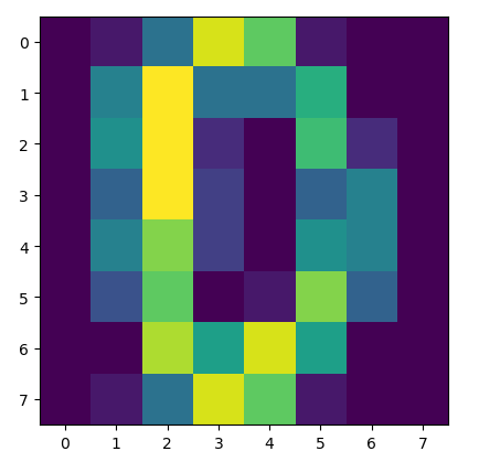
The heatmap of the handwritten digit 0 as a matrix.
Let’s standardize just this single matrix:
A_standardized = StandardScaler().fit_transform(A)

>> print(A_standardized)
>> [[0.  -1.06503581 -1.62006839  1.53587336  1.04621744 -1.48609575 -0.87576054  0.]
    [0.   0.97983294  0.92121536 -0.11461742  0.0418487   0.65388213 -0.87576054  0.]
    [0.   1.3206444   0.92121536 -0.84816887 -0.96252004  0.89165745 -0.20851441  0.]
    [0.   0.29821003  0.92121536 -0.66478101 -0.96252004 -0.53499447  1.4596009   0.]
    [0.   0.97983294  0.15883023 -0.66478101 -0.96252004  0.17833149  1.4596009   0.]
    [0.  -0.04260143 -0.09529814 -1.2149446  -0.79512525  1.36720809  0.79235477  0.]
    [0.  -1.40584727  0.41295861  0.43554618  1.54840181  0.41610681 -0.87576054  0.]
    [0.  -1.06503581 -1.62006839  1.53587336  1.04621744 -1.48609575 -0.87576054  0.]]
The data within this matrix has been standardized, and as expected, the first and last rows of the matrix are identical. This makes sense.
However, when the standardization is applied to a data frame where each row is 64 elements (not yet reshaped into the matrices), then we will obtain different values for the first and last row, and thus lose the fact that they were the same to begin with. If you look closely you’ll also see that just about every value is modified in some way. Look at how many different values a 0 is mapped to. This results in information loss and inconsistencies. Here is data and visualizations to show you what I mean:
# standardization code applied to original matrix
# df has shape (3824, 64) - it's loaded from the UCI repo linked above
df_standardized = StandardScaler().fit_transform(df)

# standardized matrix (after applying reshape)
>> print(df_standardized)
>> [[ 0.          0.80578762  0.11187895  0.7497641   0.12088469 -0.80258942 -0.41150365 -0.13531434]
    [-0.02362608  1.65043237  0.99751962 -1.42414335 -0.96579085  0.28715148 -0.54158643 -0.15369919]
    [-0.04146545  1.56407133  1.09041258 -0.79999761 -1.16971881  0.46912891 -0.01285329 -0.11292825]
    [-0.03235924  0.86332244  1.10309145 -1.03900115 -1.53914462 -0.47773704  1.28524666 -0.04857066]
    [-0.03618347  1.54299058  0.85310324 -1.00759414 -1.74717613 -0.20412106  1.17220826  0.        ]
    [-0.08686248  0.88406629  0.85202866 -1.11084563 -1.09563608  0.74489842  0.34094767 -0.09304005]
    [-0.06609584 -0.40816886  1.08179006 -0.17226062  0.98485692 -0.04768401 -0.76374843 -0.19317477]
    [-0.01617327  0.77217283  0.02894122  0.7051445   0.10769183 -0.98683408 -0.52270658 -0.17571686]]
Notice that after the standardization occurs the first and last rows are no longer the same, even though they had the same data to start with.
You can see this visually here:
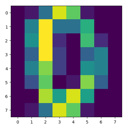
The heatmap of the matrix pre-standardization.
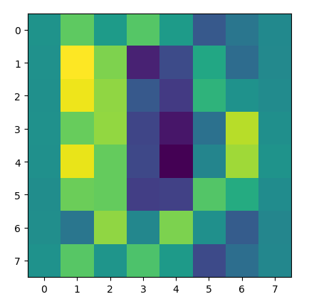
The heatmap of the matrix post-standardization.
Notice how the colors change in different places (look at the first and last row closely), indicating that the standardization has altered the matrix in a way that did not retain the original properties of the data.
I’m going to apply a row-based standardization calculation that scales the numbers but keeps their relative magnitudes by row the same.
# new standardization code applied to original matrix
# df has shape (3824, 64) - it's loaded from the UCI repo linked above
df_standardized = (df.T / df.T.sum()).T

# standardized matrix (after applying reshape)
>> [[0.  0.00322581  0.01935484  0.0483871   0.03870968  0.00322581  0.          0.]
    [0.  0.02258065  0.0516129   0.01935484  0.01935484  0.03225806  0.          0.]
    [0.  0.02580645  0.0516129   0.00645161  0.          0.03548387  0.00645161  0.]
    [0.  0.01612903  0.0516129   0.00967742  0.          0.01612903  0.02258065  0.]
    [0.  0.02258065  0.04193548  0.00967742  0.          0.02580645  0.02258065  0.]
    [0.  0.01290323  0.03870968  0.          0.00322581  0.04193548  0.01612903  0.]
    [0.  0.          0.04516129  0.02903226  0.0483871   0.02903226  0.          0.]
    [0.  0.00322581  0.01935484  0.0483871   0.03870968  0.00322581  0.          0.]]
Let’s consider the performance of the PCA’d data using a SVC just as the author in [1] did.
PCA Performance Review
In [1], using an SVC model, the author achieved a 2-Component PCA Accuracy of 55.20%. It’s interesting to note that without using any data standardization technique the 2-Component PCA Accuracy is 61.38%. This indicates that the standardization process might be hurting more than it’s helping. This is the effect I was referring to in the Introduction as “information loss”.
When the row-based standardization process is used the 2-Component PCA Accuracy is 61.83%. I double-checked the numbers and yes, the digits did indeed swap places ( .38 -> .83).
This standardization might be a better choice for the data we are considering for this problem. Let’s apply the loop written in [1] to non-standardized, and row-standardized data.
Best Accuracy according to [1]: 29-component PCA: MSE = 0.1177, Accuracy = 97.05%.
Best Accuracy according to no-standardization: 26-component PCA: MSE = 7391, Accuracy = 98.55%.
Best Accuracy according to row-standardization: 24-component PCA: MSE = 0.08607, Accuracy = 98.66%.
There is only a small difference between standardizing the data and not standardizing the data. However, it appears that on average when considering the number of components used in PCA the technique applied in [1] results in lower accuracy levels overall.
Conclusion
The purpose of [1] wasn’t to push the performance of their model, but rather to help explain the concept of PCA with a classic example. The author did a great job of that. I just wanted to explore the standardization technique they chose, and I wanted to see how things changed when using an algorithm that retained the relative values of the original data. It’s best to always consider any and all transformations we make to our data, and scrutinize whether or not they are making a positive impact on our results.
Sources
[1] https://charlesreid1.github.io/circe/Digit%20Classification%20-%20PCA%20and%20SVC.html
[2] https://archive.ics.uci.edu/ml/datasets/Optical+Recognition+of+Handwritten+Digits
Project Code
# this project comes from here: https://charlesreid1.github.io/circe/Digit%20Classification%20-%20PCA%20and%20SVC.html

import matplotlib.pyplot as plt
from matplotlib.pyplot import *
import pandas as pd
import seaborn as sns
from sklearn.preprocessing import StandardScaler
from sklearn.decomposition import PCA
from sklearn.svm import SVC
from sklearn.metrics import confusion_matrix

desired_width = 320
pd.set_option('display.width', desired_width)
np.set_printoptions(linewidth=desired_width)

testing_df = pd.read_csv('c:/users/JOSEPH~1/desktop/root/projects/_data_warehouse/optdigits.tes', header=None)
X_testing,  y_testing = testing_df.loc[:, 0:63],  testing_df.loc[:, 64]

training_df = pd.read_csv('c:/users/JOSEPH~1/desktop/root/projects/_data_warehouse/optdigits-mod.tra', header=None)
X_training, y_training = training_df.loc[:, 0:63], training_df.loc[:, 64]

print('X_training', type(X_training), X_training.shape)
print('y_training', type(y_training), y_training.shape)

matrix = X_training.loc[0, :].values.reshape(8, 8)
print(matrix, y_training[0])
plt.imshow(matrix)
gca().grid(False)
plt.show()


def get_normed_mean_cov(X):
    #X_standardized = StandardScaler().fit_transform(X)
    X_standardized = (X.T / X.T.sum()).T
    #X_standardized = X

    X_mean = np.mean(X_standardized, axis=0)

    # Automatic:
    # X_cov = np.cov(X_standardized.T)

    # Manual:
    X_cov = (X_standardized - X_mean).T.dot((X_standardized - X_mean)) / (X_standardized.shape[0] - 1)

    return X_standardized, X_mean, X_cov


X_standardized, X_mean, X_cov = get_normed_mean_cov(X_training)
X_standardized_validation, _, _ = get_normed_mean_cov(X_testing)

print(len(X_standardized), len(X_mean), len(X_cov))

mat2 = X_standardized.loc[0, :].values.reshape(8, 8)
#mat2 = X_standardized[0].reshape(8, 8)
print(mat2)
plt.imshow(mat2)
gca().grid(False)
plt.show()

# Make PCA
pca2 = PCA(n_components=2, whiten=True)
pca2.fit(X_standardized)
X_reduced = pca2.transform(X_standardized)

print(X_reduced)

# Make SVC
linclass2 = SVC()
linclass2.fit(X_reduced, y_training)

# To color each point by the digit it represents,
# create a color map with 10 elements (10 RGB values).
# Then, use the system response (y_training), which conveniently
# is a digit from 0 to 9.


def get_cmap(n):
    #colorz = plt.cm.cool
    colorz = plt.get_cmap('Set1')
    return [colorz(float(i)/n) for i in range(n)]


colorz = get_cmap(10)
colors = [colorz[yy] for yy in y_training]

scatter(X_reduced[:, 0], X_reduced[:, 1],
        color=colors, marker='*')
xlabel("Principal Component 0")
ylabel("Principal Component 1")
title("Handwritten Digit Data in\nPrincipal Component Space",size=14)
show()

# Now see how good it is:
# Use the PCA to fit the validation data,
# then use the classifier to classify digits.
X_reduced_validation = pca2.transform(X_standardized_validation)
yhat_validation = linclass2.predict(X_reduced_validation)

y_validation = y_testing

pca2_cm = confusion_matrix(y_validation, yhat_validation)
sns.heatmap(pca2_cm, square=True, cmap='inferno')
title('Confusion Matrix:\n2-Component PCA + SVC')
ylabel('True')
xlabel('Predicted')
show()

total = pca2_cm.sum(axis=None)
correct = pca2_cm.diagonal().sum()
print("2-Component PCA Accuracy: %0.2f %%" % (100.0*correct/total))

# MSE associated with back-projection:
X_orig = X_standardized
X_hat = pca2.inverse_transform(pca2.transform(X_orig))
print(X_hat)
print(X_hat.shape, X_orig.shape)

mse = sum(((X_hat - X_orig)**2).mean(axis=None))*100
#mse = ((X_hat - X_orig)**2).mean(axis=None)
print(mse)

# Make PCA
pca5 = PCA(n_components=5, whiten=True)
pca5.fit(X_standardized)
X_reduced = pca5.transform(X_standardized)

# Make SVC
linclass5 = SVC()
linclass5.fit(X_reduced, y_training)

# Use the PCA to fit the validation data,
# then use the classifier to classify digits.
X_reduced_validation = pca5.transform(X_standardized_validation)
yhat_validation = linclass5.predict(X_reduced_validation)

y_validation = y_testing

pca5_cm = confusion_matrix(y_validation, yhat_validation)
sns.heatmap(pca5_cm, square=True, cmap='inferno')
title('Confusion Matrix:\n5-Component PCA + SVC')
show()

total = pca5_cm.sum(axis=None)
correct = pca5_cm.diagonal().sum()
print("5-Component PCA Accuracy: %0.2f %%" % (100.0*correct/total))


def pca_mse_accuracy(n):
    """
    Creates a PCA model with n components,
    reduces the dimensionality of the validation data set,
    then computes two error metrics:
    * Percent correct predictions using linear classifier
    * Back-projection error (MSE of back-projected X minus original X)
    """

    X_std, _, _ = get_normed_mean_cov(X_training)
    X_std_validation, _, _ = get_normed_mean_cov(X_testing)

    #########
    # Start by making PCA/SVC
    # Train on training data

    # Make PCA
    pca = PCA(n_components=n, whiten=True)
    pca.fit(X_std)
    X_red = pca.transform(X_std)

    # Make SVC
    linclass = SVC()
    linclass.fit(X_red, y_training)

    ########
    # Now transform validation data

    # Transform inputs and feed them to linear classifier
    y_validation = y_testing
    X_red_validation = pca.transform(X_std_validation)
    yhat_validation = linclass.predict(X_red_validation)

    # Evaluate confusion matrix for predictions
    cm = confusion_matrix(y_validation, yhat_validation)
    total = cm.sum(axis=None)
    correct = cm.diagonal().sum()
    accuracy = 1.0 * correct / total

    # MSE associated with back-projection:
    X_orig = X_std
    X_hat = pca.inverse_transform(pca.transform(X_orig))
    mse = sum(((X_hat - X_orig) ** 2).mean(axis=None))*100

    return mse, accuracy


mses = []
accuracies = []
N = 33
for i in range(1, N):
    m, a = pca_mse_accuracy(i)

    print("%d-component PCA: MSE = %0.4g, Accuracy = %0.2f" % (i, m, a * 100.0))

    mses.append((i, m))
    accuracies.append((i, a))

mses = np.array(mses)
accuracies = np.array(accuracies)

# Now plot the accuracy
plt.plot(accuracies[:, 0],accuracies[:, 1], 'bo-')
plt.title("Percent Correct: Accuracy of Predictions", size=14)
plt.xlabel("Number of Principal Components")
plt.ylabel("Percent Correct")
plt.show()

# MSE, PCA Plot
Nmax = 64
pcafull = PCA(n_components=Nmax, whiten=True)
_ = pcafull.fit(X_standardized)
explained_var_sum = pcafull.explained_variance_.sum()

explained_var = np.cumsum(pcafull.explained_variance_[:N])
explained_var /= explained_var_sum

plot(mses[:, 0], mses[:, 1], '-o', label='MSE')
plot(mses[:, 0], 1.0-mses[:, 1], '-o', label='1.0 - MSE')
plot(range(1, len(explained_var)+1), explained_var, '-o', label='Expl Var')

xlabel('Number of Principal Components')
ylabel('')
title('Mean Square Error, Principal Components Analysis')

legend(loc='best')
show()
Leave a Reply